- 대회설명: Dacon 웹 로그 데이터를 활용하여 앞으로 한 달 간 사용자의 로그인 여부를 예측
- 대회일자: 2019.08.05 ~ 2019.09.05
- 주관: Dacon
- 수상실적: 1위
import pandas as pd
import numpy as np
import seaborn as sns
import matplotlib.pyplot as plt
import warnings
plt.style.use('fivethirtyeight')
warnings.filterwarnings('ignore')
데이터
import os
os.chdir('C:\\Users\\Kim\\Desktop\\TNT\\웹데이터')
train = pd.read_csv('train.csv')
test = pd.read_csv('test.csv')
TNT = pd.concat([train, test], axis = 0)
TNT.head() #Feature 파악
| Sex | apple_rat | email_type | login | past_1_month_login | past_1_week_login | past_login_total | person_id | phone_rat | sub_size | |
|---|---|---|---|---|---|---|---|---|---|---|
| 0 | male | 1.0 | naver | 0.0 | 0.0 | 0.0 | 1.0 | 1015 | 0.0 | 0.0 |
| 1 | female | 1.0 | other | 0.0 | 0.0 | 0.0 | 2.0 | 1940 | 1.0 | 0.0 |
| 2 | male | 0.0 | other | 0.0 | 0.0 | 0.0 | 1.0 | 1356 | 1.0 | 0.0 |
| 3 | male | 1.0 | other | 0.0 | 0.0 | 0.0 | 2.0 | 1535 | 0.0 | 0.0 |
| 4 | female | 0.0 | naver | 0.0 | NaN | NaN | NaN | 216 | 0.0 | 0.0 |
#Nan값 파악
TNT.isnull().sum()
Sex                     0
apple_rat               0
email_type              0
login                 682
past_1_month_login    227
past_1_week_login     227
past_login_total      227
person_id               0
phone_rat               0
sub_size                0
dtype: int64
#nan값 시각화
import missingno as msno
msno.matrix(TNT)
plt.show()

#Feature 정보 파악
TNT.info()
<class 'pandas.core.frame.DataFrame'>
Int64Index: 2182 entries, 0 to 681
Data columns (total 10 columns):
Sex                   2182 non-null object
apple_rat             2182 non-null float64
email_type            2182 non-null object
login                 1500 non-null float64
past_1_month_login    1955 non-null float64
past_1_week_login     1955 non-null float64
past_login_total      1955 non-null float64
person_id             2182 non-null int64
phone_rat             2182 non-null float64
sub_size              2182 non-null float64
dtypes: float64(7), int64(1), object(2)
memory usage: 187.5+ KB
#전체적인 통계파악
TNT.describe()
| apple_rat | login | past_1_month_login | past_1_week_login | past_login_total | person_id | phone_rat | sub_size | |
|---|---|---|---|---|---|---|---|---|
| count | 2182.000000 | 1500.000000 | 1955.000000 | 1955.000000 | 1955.000000 | 2182.000000 | 2182.000000 | 2182.000000 |
| mean | 0.220114 | 0.099333 | 0.607161 | 0.257801 | 7.702813 | 1091.489918 | 0.125673 | 2.976169 |
| std | 0.397746 | 0.299209 | 3.215901 | 1.301143 | 21.546863 | 630.050764 | 0.295775 | 15.481671 |
| min | 0.000000 | 0.000000 | 0.000000 | 0.000000 | 1.000000 | 0.000000 | 0.000000 | 0.000000 |
| 25% | 0.000000 | 0.000000 | 0.000000 | 0.000000 | 1.000000 | 546.250000 | 0.000000 | 0.000000 |
| 50% | 0.000000 | 0.000000 | 0.000000 | 0.000000 | 2.000000 | 1091.500000 | 0.000000 | 0.000000 |
| 75% | 0.126995 | 0.000000 | 0.000000 | 0.000000 | 5.000000 | 1636.750000 | 0.000000 | 0.000000 |
| max | 1.000000 | 1.000000 | 93.000000 | 23.000000 | 503.000000 | 2182.000000 | 1.000000 | 358.000000 |
string_data = TNT.select_dtypes(include = ['object'])
int_data = TNT.select_dtypes(include = ['int64'])
float_data = TNT.select_dtypes(include = ['float64'])
#문자형 유니크 데이터 파악
for col in string_data.columns:
    print('Unique values for {0}:\n{1}\n'.format(col, string_data[col].unique()))
Unique values for Sex:
['male' 'female']

Unique values for email_type:
['naver' 'other' 'gmail' 'nate' 'hanmail']
#숫자형 유니크 데이터 파악
for col in int_data.columns:
    print('Unique values for {0}:\n{1}\n'.format(col, int_data[col].unique()))
Unique values for person_id:
[1015 1940 1356 ...  289 1590  572]
#실수형 유니크 데이터 파악
for col in float_data.columns:
    print('Unique values for {0}:\n{1}\n'.format(col, float_data[col].unique()))
Unique values for apple_rat:
[1.         0.         0.85416667 0.8        0.5        0.25
 0.08333333 0.01666667 0.4        0.76923077 0.875      0.2
 0.66666667 0.57142857 0.13157895 0.125      0.81818182 0.55555556
 0.86170213 0.21052632 0.88235294 0.16666667 0.03225806 0.92
 0.85714286 0.33333333 0.09090909 0.93877551 0.625      0.71428571
 0.75       0.26666667 0.52631579 0.70588235 0.375      0.0625
 0.91304348 0.42857143 0.13333333 0.03333333 0.15       0.83333333
 0.03703704 0.3        0.35       0.95238095 0.28571429 0.91666667
 0.11764706 0.68181818 0.6        0.07692308 0.92307692 0.05405405
 0.88888889 0.12765957 0.47368421 0.44444444 0.54545455 0.13043478
 0.07462687 0.35714286 0.14285714 0.1509434  0.90566038 0.06666667
 0.14864865 0.07142857 0.11111111 0.01630435 0.03448276 0.12922465
 0.1875     0.96666667 0.18181818 0.53333333 0.20454545 0.86666667
 0.7037037  0.27659574 0.04       0.98863636 0.91111111 0.12903226
 0.08108108 0.94736842]

Unique values for login:
[ 0.  1. nan]

Unique values for past_1_month_login:
[ 0. nan  1.  2.  5.  3.  4. 12. 18.  9. 13.  6.  7.  8. 21. 17. 50. 19.
 11. 29. 93. 26. 20. 27. 10.]

Unique values for past_1_week_login:
[ 0. nan  5.  2.  4.  1.  3.  9. 11.  6. 12. 18.  8.  7. 17. 20. 23.]

Unique values for past_login_total:
[  1.   2.  nan   4.  48.   5.  14.   3.   8.   9. 234.  12.  58.   7.
 240.  10.  24.  65.  26.  61. 139.   6.  13.  23.  20.  11.  18.  25.
  16.  38.  56.  15.  94.  19.  35.  27.  17.  31.  32.  30.  33.  62.
  98.  21.  88.  45.  76.  40.  77.  28. 115.  60.  52. 236.  22.  54.
 125. 132.  50.  37.  64. 119.  34.  39.  47.  41. 112. 117. 101.  29.
 134.  73.  53.  36.  74. 184.  81. 503.  86.  87.  44.  42.  72. 111.
  93.  68.]

Unique values for phone_rat:
[0.         1.         0.0625     0.07142857 0.5        0.25
 0.77777778 0.06837607 0.08333333 0.01666667 0.01538462 0.1
 0.4        0.07913669 0.15384615 0.15       0.42857143 0.05555556
 0.2        0.33333333 0.14285714 0.13157895 0.61538462 0.8
 0.64285714 0.86170213 0.22222222 0.08571429 0.21052632 0.23529412
 0.6        0.07692308 0.09090909 0.03225806 0.11111111 0.16666667
 0.03278689 0.01020408 0.08695652 0.03333333 0.11363636 0.75
 0.26666667 0.01315789 0.01136364 0.37037037 0.05263158 0.35
 0.1875     0.66666667 0.21875    0.09375    0.12987013 0.30434783
 0.00869565 0.09230769 0.12121212 0.03703704 0.00423729 0.05
 0.26315789 0.12962963 0.92       0.78571429 0.28571429 0.17857143
 0.015625   0.11764706 0.02272727 0.43589744 0.04878049 0.125
 0.73684211 0.04       0.92307692 0.05405405 0.03418803 0.03960396
 0.18181818 0.05714286 0.12765957 0.47368421 0.3        0.27586207
 0.04347826 0.27272727 0.17164179 0.19491525 0.08219178 0.03448276
 0.1509434  0.06666667 0.83333333 0.02941176 0.13888889 0.14864865
 0.04761905 0.95454545 0.44444444 0.13793103 0.35643564 0.76190476
 0.90909091 0.09940358 0.96666667 0.375      0.20930233 0.55263158
 0.22641509 0.03947368 0.03030303 0.0952381  0.07407407 0.4893617
 0.48611111 0.07207207 0.55       0.02857143 0.54411765 0.23076923
 0.09677419 0.52380952 0.17142857 0.30769231 0.11538462 0.71428571
 0.14814815 0.08108108 0.12068966]

Unique values for sub_size:
[  0.  28. 139.   3.   1. 114.   9.   6.  95.  56.   5. 163.  25.  17.
  10.   8.   7.   2.  76.  20.   4.  46. 100.  19.  15.  34.  12.  49.
 358. 149.  32.  43.  30.  13.  11.  80.  81.  23.  37.  82.  62. 166.
  24.  16.  18.  26.  41.  50.  96.  55. 110.  33.  21.  91.  14.  29.
  39. 282.  99.  63.  27.  36.  44.  68.  53.  45. 101.  64.  78.  22.
 140.  38.  35.  48.  59.]
EDA
http://newsjel.ly/archives/newsjelly-report/visualization-report/8136(데이터 특징별 그래프 선택 방법)
plt.figure(figsize = [15,8])
sns.kdeplot(TNT.apple_rat, label = 'apple_rat')
plt.show()

TNT.apple_rat.hist()
<matplotlib.axes._subplots.AxesSubplot at 0xa383ed2710>
plt.figure(figsize = [15,8])
sns.kdeplot(TNT.apple_rat, label = 'phone_rat')
plt.show()

TNT.phone_rat.hist()
<matplotlib.axes._subplots.AxesSubplot at 0xa382897d30>
plt.figure(figsize = [15,8])
sns.kdeplot(TNT.apple_rat, label = 'sub_size')
plt.show()
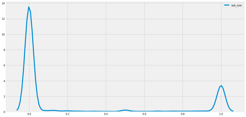
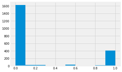
TNT.sub_size.hist()
<matplotlib.axes._subplots.AxesSubplot at 0xa383df1cc0>

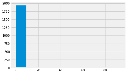
sns.countplot(TNT['sub_size'])
<matplotlib.axes._subplots.AxesSubplot at 0xa383d9a710>

plt.figure(figsize = [15,8])
sns.kdeplot(TNT.past_1_month_login, label = 'past_1_month_login')
plt.show()
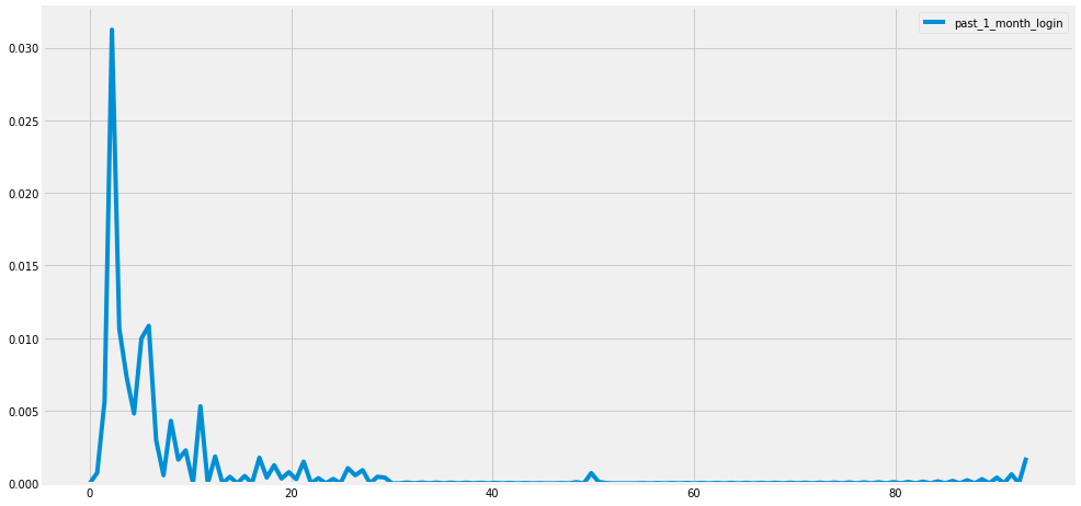
TNT.past_1_month_login.hist()
<matplotlib.axes._subplots.AxesSubplot at 0xa383e28320>
sns.countplot(TNT['past_1_month_login'])
<matplotlib.axes._subplots.AxesSubplot at 0xa383e90470>

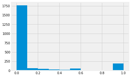
plt.figure(figsize = [15,8])
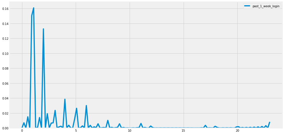
sns.kdeplot(TNT.past_1_week_login, label = 'past_1_week_login')
plt.show()
TNT.past_1_week_login.hist()
<matplotlib.axes._subplots.AxesSubplot at 0xa3840c7a58>

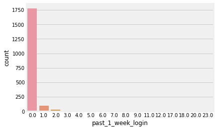
sns.countplot(TNT['past_1_week_login'])
<matplotlib.axes._subplots.AxesSubplot at 0xa38412d630>
plt.figure(figsize = [15,8])
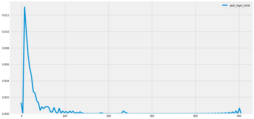
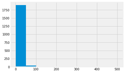
sns.kdeplot(TNT.past_login_total, label = 'past_login_total')
plt.show()
TNT.past_login_total.hist()
<matplotlib.axes._subplots.AxesSubplot at 0xa384415be0>
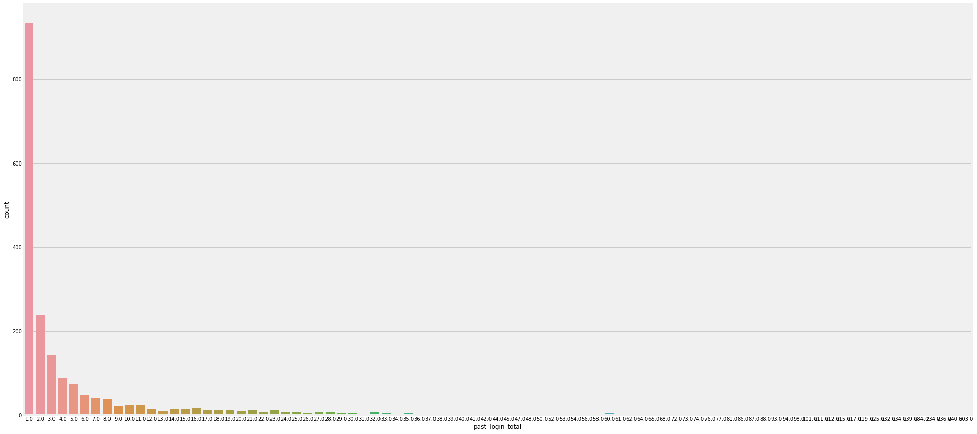
plt.figure(figsize = [30,15])
sns.countplot(TNT['past_login_total'])
<matplotlib.axes._subplots.AxesSubplot at 0xa38444b550>
전처리
from sklearn.preprocessing import LabelEncoder
label = LabelEncoder()
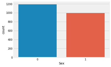
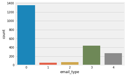
for col in ["Sex", 'email_type']:
TNT[col] = label.fit_transform(TNT[col])
sns.countplot(TNT['Sex'])
<matplotlib.axes._subplots.AxesSubplot at 0x14e3cccd68>
sns.countplot(TNT['email_type'])
<matplotlib.axes._subplots.AxesSubplot at 0x9432400908>
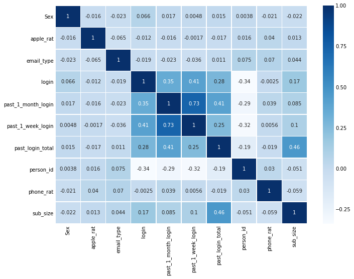
sns.heatmap(TNT.corr(),annot=True,cmap='Blues',linewidths=0.5) #annot - 빈칸에 상관계수 채워줌
fig=plt.gcf()
fig.set_size_inches(10,8)
plt.show()
TNT.head()
| Sex | apple_rat | email_type | login | past_1_month_login | past_1_week_login | past_login_total | person_id | phone_rat | sub_size | |
|---|---|---|---|---|---|---|---|---|---|---|
| 0 | 1 | 1.0 | 3 | 0.0 | 0.0 | 0.0 | 1.0 | 1015 | 0.0 | 0.0 |
| 1 | 0 | 1.0 | 4 | 0.0 | 0.0 | 0.0 | 2.0 | 1940 | 1.0 | 0.0 |
| 2 | 1 | 0.0 | 4 | 0.0 | 0.0 | 0.0 | 1.0 | 1356 | 1.0 | 0.0 |
| 3 | 1 | 1.0 | 4 | 0.0 | 0.0 | 0.0 | 2.0 | 1535 | 0.0 | 0.0 |
| 4 | 0 | 0.0 | 3 | 0.0 | NaN | NaN | NaN | 216 | 0.0 | 0.0 |
——————————————————-
TNT['MAC_OS'] = TNT['phone_rat']-TNT['apple_rat']
TNT.drop(['phone_rat', 'past_login_total' ], axis = 1, inplace = True) #열제거
TNT['past_1_month_login'] = TNT['past_1_month_login'].fillna(0.6)
TNT['past_1_week_login'] = TNT['past_1_week_login'].fillna(0.25)
——————————————————
결측치를 바꾸거나 Feature Engineering을 시도 했었는데 결과가 좋지 않아 사용하지 않았음
#데이터 분리
train = TNT.loc[TNT.login.notnull()]
test = TNT.loc[TNT.login.isna()]
#모델에 넣을 train 확인
train.info()
<class 'pandas.core.frame.DataFrame'>
Int64Index: 1500 entries, 0 to 1499
Data columns (total 9 columns):
Sex                   1500 non-null int64
apple_rat             1500 non-null float64
email_type            1500 non-null int64
login                 1500 non-null float64
past_1_month_login    1340 non-null float64
past_1_week_login     1340 non-null float64
person_id             1500 non-null int64
sub_size              1500 non-null float64
MAC_OS                1500 non-null float64
dtypes: float64(6), int64(3)
memory usage: 117.2 KB
모델링
참고 https://www.kaggle.com/lifesailor/xgboost
from sklearn.model_selection import GridSearchCV
import xgboost as xgb
from xgboost.sklearn import XGBRegressor
from sklearn import metrics
def modelfit(alg, x_train, y_train,useTrainCV=True, cv_folds=5, early_stopping_rounds=100):

    if useTrainCV:
        xgb_param = alg.get_xgb_params()
        xgtrain = xgb.DMatrix(x_train, label=y_train)
        cvresult = xgb.cv(xgb_param, xgtrain, num_boost_round=alg.get_params()['n_estimators'], nfold=cv_folds,
                          metrics='rmse', early_stopping_rounds=early_stopping_rounds)
        alg.set_params(n_estimators=cvresult.shape[0])
        print(alg)


    alg.fit(x_train, y_train, eval_metric='rmse')


    dtrain_predictions = alg.predict(x_train)

    #Print model report:
    print("\nModel Report")
    print("Training Accuracy : %.4g" % metrics.mean_squared_error(y_train, dtrain_predictions))
#처음 min_child_weight를 5로 설정했을 때 변화
#두번째 scale_pos_weight를 5로 설정했을 때 변화
# scale_pos_weight를 6으로 했을 때 변화
xgb1 = XGBRegressor(
    learning_rate =0.2,  #Learning rate(일반적으로 0.01 - 0.2)
    n_estimators=5000,
    max_depth=2,   #tree 깊이
    min_child_weight=5,  # min_child_weight를 기준으로 추가 분기 결정(크면 Underfitting)
    gamma=0,   #split 하기 위한 최소의 loss 감소 정의
    subsample=0.6,  #데이터 중 샘플링(0.5 - 1)
    colsample_bytree=0.6, #column 중 sampling(0.5 - 1)
    objective= "binary:logistic",
    nthread=-1,  #병렬 처리 조절
    scale_pos_weight=6, #positive, negative weight 지정
    seed=2018  #모델이 매번 수행시, 샘플링 결과가 바뀔수 있으므로 지정
)
modelfit(xgb1, train.drop(['login'],axis = 1), train['login'])
XGBRegressor(base_score=0.5, booster='gbtree', colsample_bylevel=1,
       colsample_bynode=1, colsample_bytree=0.6, gamma=0,
       importance_type='gain', learning_rate=0.2, max_delta_step=0,
       max_depth=2, min_child_weight=5, missing=None, n_estimators=55,
       n_jobs=1, nthread=-1, objective='binary:logistic', random_state=0,
       reg_alpha=0, reg_lambda=1, scale_pos_weight=6, seed=2018,
       silent=None, subsample=0.6, verbosity=1)

Model Report
Training Accuracy : 0.0905
제출
submission = pd.DataFrame({'person_id': test['person_id'] , 'login' : xgb1.predict(test.drop(['login'], axis = 1))})
submission.to_csv('submission9.csv', index = False)