- 대회설명: Statcast 데이터 중심의 구종 개수와 아웃 확률에 기반한 투수 평가
- 대회일자: 2019.03.25 ~ 2019.05.20
- 주관: Dacon
-
수상실적: 1위
- 이미지를 클릭하시면 방법론 및 코드 설명 영상이 재생됩니다.

Statcast 데이터 중심의 구종 개수와 아웃 확률에 기반한 투수 평가
문제 정의
- 2019년에 새로 뽑힌 13명의 외국인 투수 중 2명을 스카우트
어떻게 문제를 해결할 것인가?
- KBO에서 “좋은 활약”을 보였던 외국인 투수 중, 그들이 한국에 오기 전 MLB에서의 “특성”을 찾아내어, 그것과 유사한 특징을 보이고 있는 투수 2명을 스카우트 하자
단어 정의
-
KBO에서 “좋은 활약”: TBF가 중앙값 이상이고 (충분한 시행 횟수), ERA가 중앙값 이하인 집단
- 각 지표들의 variance가 커서, 평균 보다는 중앙값이 기준점으로 타당하다고 판단하였다.
-
특성: 구종의 개수와 아웃 확률
-
구종의 개수
-
최근 류현진이 MLB에서 제구력이 높은 다양한 구종들을 구사하며 좋은 투수로써 평가를 받고 있는 점에 기반하여 특성으로 쓰기로 하였다.
-
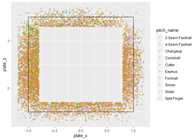
표본공간: strike zone의 edge 부분에서 던진 공 중에서 strike 판정을 받은 공
-
strike zone (xlim = c(-1,1), ylim = c(1.5, 3.5))
-
edge부분은 strike zone으로 부터 x축 y축 각각 +- 0.2로 계산하였다.
-
edge 조건은 “제구력”이라는 개념을 반영하기 위해서 추가 하였다.
-
-
해당 표본공간에서 각 구종별 비율을 계산하였을 때, 비율이 0.1 이상의 공이 해당 투수가 자유롭게 구사할 수 있는 공이라고 판단하였다.
-
-
아웃 확률
-
아웃 확률이라는 개념은, 기존에 집계된 전통적인 데이터로부터는 도출 할 수 없는 개념이다.
-
허나 Statcast 데이터를 통해서 해당 개념을 나타낼 수 있기 때문에 활용하기로 하였다.
-
“Modeling Pitcher Performance and the Distribution of Runs per Inning in Major League Baseball”(1996)에 나오는 아웃 확률 추정 공식을 사용하였다.
-
-
스카우트 기준
- 11.18 집단을 통해 구종의 개수가 증가할 때 마다 ERA가 유의미하게 감소하는 경향이 확인된다면, 19년도 투수 중 구종의 개수가 가장 많은 집단 내에서 아웃 확률이 가장 높은 투수 2명을 스카우트 할 것이다.
시각화
- 해당 실험에 대한 아이디어를 얻기 위해 대부분의 시각화는 Tableau로 진행하였다.
# library 로드
library(tidyverse)
#데이터셋 불러오기
atKbo.11.18.KboRegSsn <- read_csv("./datasets/kbo_yearly_foreigners_2011_2018.csv")

atKbo.11.18.MlbTot <- read_csv("./datasets/fangraphs_foreigners_2011_2018.csv")

atKbo.11.18.StatCast <- read_csv("./datasets/baseball_savant_foreigners_2011_2018.csv")

atKbo.19.MlbTot <- read_csv("./datasets/fangraphs_foreigners_2019.csv")

atKbo.19.StatCast <- read_csv("./datasets/baseball_savant_foreigners_2019.csv",
                              guess_max = 2000) # guess_max 세팅하지 않으면 parsing 오류 발생
# 비교 가능한 그룹 선정하기

## 데이터셋을 확인해보니, KBO성적은 있으나 MLB 성적이 없는 경우, MLB 성적은 있으나 KBO 성적이 없는 경우, 등등 예외적인 pitcher들이 존재하였다.

## 원활한 비교를 위해, 각 데이터셋 별로 공통적으로 있는 pitcher들을 먼저 골라내보겠다.
target <- intersect(unique(atKbo.11.18.KboRegSsn$pitcher_name),
                    unique(atKbo.11.18.MlbTot$pitcher_name)) %>%
    intersect(unique(atKbo.11.18.StatCast$pitcher_name))

target %>% length()
## [1] 57
intersect(unique(atKbo.11.18.KboRegSsn$pitcher_name),
                    unique(atKbo.11.18.MlbTot$pitcher_name)) %>% length()
## [1] 59
# 구단 입장에서는 투수가 온 첫번째 해에 의미있는 성적을 기대할 것이라고 판단하여, 외국인 투수들의 KBO 첫 시즌 기록을 따로 추출하였음.

firstYearInKBO.11.18 <- atKbo.11.18.KboRegSsn %>%
    filter(pitcher_name %in% target) %>%
    group_by(pitcher_name) %>%
    filter(year == min(year)) # 투수별 year에서 가장 적은 값 = 첫 시즌
# 해당 데이터에서 TBF가 중앙값 이상, ERA가 중앙값 이하인 Elite 그룹을 선정

Elite.11.18 <- firstYearInKBO.11.18 %>%
    filter(TBF >= median(firstYearInKBO.11.18$TBF) & ERA <= median(firstYearInKBO.11.18$ERA))
구종 개수
# 선수별 구종 개수 feature 만들기
# 구종 개수 대한 정의는 서론 참조

atKbo.11.18.StatCast$pitch_name %>% unique()
##  [1] "4-Seam Fastball"  "Changeup"         "2-Seam Fastball"  "Curveball"
##  [5] NA                 "Cutter"           "Intentional Ball" "Slider"
##  [9] "Pitch Out"        "Forkball"         "Sinker"           "Unknown"
## [13] "Eephus"           "Fastball"         "Split Finger"
coordEdge <- atKbo.11.18.StatCast %>%
    filter((plate_x >= 0.8 & plate_x <= 1.2 & plate_z <= 3.7 & plate_z >= 1.3) |  # edge 영역 안에 있는 투구 추출
               (plate_x <= -0.8 & plate_x >= -1.2 & plate_z <= 3.7 & plate_z >= 1.3) |
               (plate_x >= -0.8 & plate_x <= 0.8 & plate_z <= 1.7 & plate_z >= 1.3) |
               (plate_x >= -0.8 & plate_x <= 0.8 & plate_z <= 3.7 & plate_z >= 3.3)) %>%
    filter(pitch_name != is.na(pitch_name)) %>% # pitch 이름이 기록 안된 것 제거
    filter(pitch_name != "Intentional Ball") %>% # 고의사구 제거
    filter(description == "called_strike") %>% # strike인 것만 추출
    group_by(pitcher_name, pitch_name) %>%
    summarise(n = n()) %>%
    ungroup() %>%
    group_by(pitcher_name) %>%
    mutate(totalEdges = sum(n),
           byPitchPercentage = n / totalEdges) %>%
    filter(byPitchPercentage >= 0.1) %>%
    summarise(numberofPitches = n()) %>%
    ungroup()
# edge에 있는 투구 시각화 예시

atKbo.11.18.StatCast %>%
    filter((plate_x >= 0.8 & plate_x <= 1.2 & plate_z <= 3.7 & plate_z >= 1.3) |  # edge 영역 안에 있는 투구 추출
               (plate_x <= -0.8 & plate_x >= -1.2 & plate_z <= 3.7 & plate_z >= 1.3) |
               (plate_x >= -0.8 & plate_x <= 0.8 & plate_z <= 1.7 & plate_z >= 1.3) |
               (plate_x >= -0.8 & plate_x <= 0.8 & plate_z <= 3.7 & plate_z >= 3.3)) %>%
    filter(pitch_name != is.na(pitch_name)) %>% # pitch 이름이 기록 안된 것 제거
    filter(pitch_name != "Intentional Ball") %>% # 고의사구 제거
    filter(description == "called_strike") %>% # strike인 것만 추출
    ggplot(aes(x = plate_x, y = plate_z)) +
    geom_point(aes(col = pitch_name), alpha = 0.3) +
    geom_rect(aes(xmin = -1, xmax = 1, ymin = 1.5, ymax = 3.5), alpha = 0, color = "black")
#Elite 그룹 데이터 셋에, 구종 개수 feature 추가

coordEdgeJoin <- inner_join(Elite.11.18, coordEdge, by = "pitcher_name")
# 구종 개수 별, ERA의 박스플롯 시각화


coordEdgeJoin %>%
    ggplot(aes(x = numberofPitches, y = ERA)) +
    geom_boxplot(aes(group = numberofPitches)) +
    ylab(label = "ERA of First Season in KBO") +
    geom_point()

lm(ERA ~ numberofPitches, data = coordEdgeJoin) %>% summary()
##
## Call:
## lm(formula = ERA ~ numberofPitches, data = coordEdgeJoin)
##
## Residuals:
##     Min      1Q  Median      3Q     Max
## -1.1344 -0.2762 -0.1009  0.4348  0.8956
##
## Coefficients:
##                 Estimate Std. Error t value Pr(>|t|)
## (Intercept)       4.7731     0.4135  11.543  3.6e-09 ***
## numberofPitches  -0.3629     0.1499  -2.421   0.0277 *
## ---
## Signif. codes:  0 '***' 0.001 '**' 0.01 '*' 0.05 '.' 0.1 ' ' 1
##
## Residual standard error: 0.5664 on 16 degrees of freedom
## Multiple R-squared:  0.2681,	Adjusted R-squared:  0.2224
## F-statistic: 5.861 on 1 and 16 DF,  p-value: 0.02773
-
확인 결과, Elite 그룹에서는 구종의 개수가 증가 할 수록, KBO에서의 첫 시즌 ERA가 줄어드는 모습을 보이고 있다.
-
그렇기 때문에 구종의 개수가 많은 투수를 우선적으로 선택할 것이다.
아웃 확률 추정하기
-
참고문헌에 의하면 아웃 확률을 추정하기 위해선 이닝별로 상대한 타자의 수에 대한 정보가 필요하다
-
StatCast에는 정확한 이닝별 기록이 없다.
-
그래서 이닝별로 상대한 타자의 수를 만들기 위해, events에 “out”이 포함된 값들을 활용하여 해당 경기에 이닝에 대한 정보를 구하였다.
-
events의 out을 기준으로 이닝을 구분하였고, 해당 이닝에 상대한 타자의 수를 구하였다.
-
만약 투수가 이닝을 끝내지 못하고 중도 교체를 당하면, 교체 당하기 전까지 상대한 타자의 수에 남은 아웃 카운트를 더하여 “이닝별로 상대한 타자의 수”를 추정하였다.
# 우선 한 이닝에 가장 많이 상대가능 한 타자를 추정해볼 것임
# 타자 별로 오로지 하나의 "events" 값만 지니고, 나머지 값들은 NA로 기입 되어 있음
# 그렇기 때문에 events에 대해서 NA 값들을 제거 하면, 투수가 상대한 타자의 수를 알 수 있다.

atKbo.11.18.StatCast %>%
    filter(events != is.na(events)) %>% #events에 대해서 NA 값 제거
    group_by(pitcher_name, game_date) %>% #pitcher_name과 game_date 별로 그룹화
    summarise(battersfaced = NROW(pitcher_name)) %>% # 해당 투수가 해당 날짜에 상대한 타자의 수
    ungroup() %>%
    filter(battersfaced == max(battersfaced)) # 최대값
## # A tibble: 1 x 3
##   pitcher_name game_date  battersfaced
##   <chr>        <date>            <int>
## 1 레이예스     2011-05-30           36
atKbo.11.18.StatCast$events %>% unique()
##  [1] "field_out"                    "home_run"
##  [3] NA                             "single"
##  [5] "walk"                         "strikeout"
##  [7] "hit_by_pitch"                 "triple"
##  [9] "double"                       "intent_walk"
## [11] "sac_bunt"                     "sac_fly"
## [13] "force_out"                    "grounded_into_double_play"
## [15] "double_play"                  "field_error"
## [17] "fielders_choice_out"          "pickoff_caught_stealing_2b"
## [19] "fielders_choice"              "strikeout_double_play"
## [21] "caught_stealing_2b"           "other_out"
## [23] "catcher_interf"               "sac_fly_double_play"
## [25] "pickoff_1b"                   "pickoff_caught_stealing_home"
## [27] "run"
즉, 최악의 경우에는 한 이닝에 36명에 타자에 대해서 아웃을 잡지 못하고 중도 교체가 될 수 있다. 그렇게 되면 총 39명의 타자를 상대한 꼴이 된다.
# 추후에 추가할 column명 만들기
# I_N 형식 (N은 해당 이닝에 상대한 타자 수)

innings_name <- vector()


for (i in 3:39) {  #한 이닝에 최소로 상대 가능한 타자 수는 3, 최대는 위에서 구하여 39

    innings_name <- append(innings_name, paste0("I_", i))

}

innings_name
##  [1] "I_3"  "I_4"  "I_5"  "I_6"  "I_7"  "I_8"  "I_9"  "I_10" "I_11" "I_12"
## [11] "I_13" "I_14" "I_15" "I_16" "I_17" "I_18" "I_19" "I_20" "I_21" "I_22"
## [21] "I_23" "I_24" "I_25" "I_26" "I_27" "I_28" "I_29" "I_30" "I_31" "I_32"
## [31] "I_33" "I_34" "I_35" "I_36" "I_37" "I_38" "I_39"
# 데이터셋을 순회하면서 inning  별 상대한 타자 수를 저장하는 함수 만들기

fun_inningResults <- function(data) {

    # init
    batterCount <- 0 #batterCount 초기화
    inningCount <- 0 #inningCount 초기화
    batterCountTemp <- 0
    outs <- c("out", "out", "out") #out stack  초기화

    l <- list() #inning 리스트 초기화

    # inning 리스트 key 값 만들어 주고, value 값 초기화
    for (i in (1:37)) {

        l[[innings_name[i]]] <- 0

    }


    # traverse

    for (i in c(NROW(data):1)) {

        batterCount <- batterCount + 1 #traverse할 때마다 batterCount 증가

        if (grepl("out", data[i])) { #out을 만나면

            outs <- head(outs, -1) #out stack에서 pop 하기

        }

        if (length(outs) == 0) { #out이 3번 나오면

            inningCount <- inningCount + 1 #inningCount 증가

            l[[names(l)[batterCount - batterCountTemp - 2]]] <- l[[names(l)[batterCount - batterCountTemp - 2]]] + 1 #해당 I_N에 1증가

            batterCountTemp <- batterCount #추후 상대한 인원 알기 위해, batterCountTemp에 저장

            outs <- c("out", "out", "out") #out stack  초기화

        }

    }


    # out stack의 empty 유무에 따라 inning list를 마무해주자

    if (length(outs) != 0) {

        l[[names(l)[batterCount - batterCountTemp + length(outs) - 2]]] <- l[[names(l)[batterCount - batterCountTemp + length(outs) - 2]]] + 1

    }

    # inning list가 완성 되었다.

    # summarise 용 함수로 쓸 것이기 때문에, 경기별 이닝별 상대한 타자의 수에대한 정보를 한 줄로 표현하자

    # I_N&n : N = 이닝에 상대한 타자 수, n = I_N의 개수

    result = NULL

    for (i in 1:37) {

        result <- paste0(result, names(l)[i], "&", l[[names(l)[i]]], " ")

    }

    return(result)

}
# fun_inningResults 적용
statcast.11.18_inningResult <- atKbo.11.18.StatCast %>%
    filter(events != is.na(events)) %>% #events의 NA값 제거
    group_by(pitcher_name, game_date) %>%
    summarise(inningResults = fun_inningResults(events)) %>%
    ungroup()
statcast.11.18_inningResult %>% head()
## # A tibble: 6 x 3
##   pitcher_name game_date  inningResults
##   <chr>        <date>     <chr>
## 1 니퍼트       2010-06-06 "I_3&0 I_4&0 I_5&0 I_6&2 I_7&0 I_8&0 I_9&0 I_10&0 I_1~
## 2 니퍼트       2010-06-09 "I_3&0 I_4&0 I_5&0 I_6&0 I_7&1 I_8&0 I_9&0 I_10&0 I_1~
## 3 니퍼트       2010-06-17 "I_3&0 I_4&1 I_5&1 I_6&0 I_7&0 I_8&1 I_9&0 I_10&0 I_1~
## 4 니퍼트       2010-06-23 "I_3&1 I_4&1 I_5&0 I_6&1 I_7&1 I_8&0 I_9&0 I_10&0 I_1~
## 5 니퍼트       2010-06-30 "I_3&2 I_4&1 I_5&0 I_6&1 I_7&0 I_8&0 I_9&0 I_10&0 I_1~
## 6 니퍼트       2010-07-05 "I_3&0 I_4&1 I_5&0 I_6&0 I_7&0 I_8&0 I_9&0 I_10&0 I_1~
#inningResults를 parsing하여 I_N 형태에 column에 값들을 저장할 것임

#inning dataframe 만들어 주기

dataframe_inning <- as.data.frame(matrix(nrow = nrow(statcast.11.18_inningResult), ncol = 37))

colnames(dataframe_inning) <- innings_name
#inningResults에 대한 정보를 parsing 하는 함수 만들기
fun_makeInningDataset <- function(beforeParsingDataset, afterParsingDataset) {

    for (i in c(1:nrow(beforeParsingDataset))) {

        afterSplit <- strsplit(beforeParsingDataset$inningResults[i], split = " ")[[1]] %>%
            strsplit(split = "&") # " " 기준으로 parsing 한 후, "&" 기준으로 parsing 하기

        for (j in c(1:37)) {

            afterParsingDataset[i,j] <- as.numeric(afterSplit[[j]][2]) # I_N의 값 저장

        }

    }

    return(afterParsingDataset)

}

strsplit("I_3&0 I_4&0 I_5&0 I_6&2 I_7&0 I_8&0 I_9&0", split = " ")[[1]] %>%
    strsplit(split = "&")
## [[1]]
## [1] "I_3" "0"
##
## [[2]]
## [1] "I_4" "0"
##
## [[3]]
## [1] "I_5" "0"
##
## [[4]]
## [1] "I_6" "2"
##
## [[5]]
## [1] "I_7" "0"
##
## [[6]]
## [1] "I_8" "0"
##
## [[7]]
## [1] "I_9" "0"
#fun_makeInningDataset 함수 적용

dataframe_inning <- fun_makeInningDataset(beforeParsingDataset = statcast.11.18_inningResult,
                                          afterParsingDataset = dataframe_inning)
apply(dataframe_inning, 2, sum)
##  I_3  I_4  I_5  I_6  I_7  I_8  I_9 I_10 I_11 I_12 I_13 I_14 I_15 I_16 I_17 I_18
## 3731 2103 1511  981  588  318  154   75   35   13    5    2    0    1    1    0
## I_19 I_20 I_21 I_22 I_23 I_24 I_25 I_26 I_27 I_28 I_29 I_30 I_31 I_32 I_33 I_34
##    0    0    0    0    0    0    0    0    0    0    0    0    0    0    0    0
## I_35 I_36 I_37 I_38 I_39
##    0    0    0    0    0
- 18명 이상의 타자를 상대한 이닝은 존재하지 않는다. 그러므로 I_17 까지 저장하자
dataframe_inning <- dataframe_inning[,c(1:15)]
#선수가 투구한 경기별로, 이닝별 상대한 타자 수에 대한 정보를 지닌 데이터셋 생성

individualInning <- statcast.11.18_inningResult %>%
    cbind(dataframe_inning)
individualInning %>% head()
##   pitcher_name  game_date
## 1       니퍼트 2010-06-06
## 2       니퍼트 2010-06-09
## 3       니퍼트 2010-06-17
## 4       니퍼트 2010-06-23
## 5       니퍼트 2010-06-30
## 6       니퍼트 2010-07-05
##                                                                                                                                                                                                                                                  inningResults
## 1 I_3&0 I_4&0 I_5&0 I_6&2 I_7&0 I_8&0 I_9&0 I_10&0 I_11&0 I_12&0 I_13&0 I_14&0 I_15&0 I_16&0 I_17&0 I_18&0 I_19&0 I_20&0 I_21&0 I_22&0 I_23&0 I_24&0 I_25&0 I_26&0 I_27&0 I_28&0 I_29&0 I_30&0 I_31&0 I_32&0 I_33&0 I_34&0 I_35&0 I_36&0 I_37&0 I_38&0 I_39&0
## 2 I_3&0 I_4&0 I_5&0 I_6&0 I_7&1 I_8&0 I_9&0 I_10&0 I_11&0 I_12&0 I_13&0 I_14&0 I_15&0 I_16&0 I_17&0 I_18&0 I_19&0 I_20&0 I_21&0 I_22&0 I_23&0 I_24&0 I_25&0 I_26&0 I_27&0 I_28&0 I_29&0 I_30&0 I_31&0 I_32&0 I_33&0 I_34&0 I_35&0 I_36&0 I_37&0 I_38&0 I_39&0
## 3 I_3&0 I_4&1 I_5&1 I_6&0 I_7&0 I_8&1 I_9&0 I_10&0 I_11&0 I_12&0 I_13&0 I_14&0 I_15&0 I_16&0 I_17&0 I_18&0 I_19&0 I_20&0 I_21&0 I_22&0 I_23&0 I_24&0 I_25&0 I_26&0 I_27&0 I_28&0 I_29&0 I_30&0 I_31&0 I_32&0 I_33&0 I_34&0 I_35&0 I_36&0 I_37&0 I_38&0 I_39&0
## 4 I_3&1 I_4&1 I_5&0 I_6&1 I_7&1 I_8&0 I_9&0 I_10&0 I_11&0 I_12&0 I_13&0 I_14&0 I_15&0 I_16&0 I_17&0 I_18&0 I_19&0 I_20&0 I_21&0 I_22&0 I_23&0 I_24&0 I_25&0 I_26&0 I_27&0 I_28&0 I_29&0 I_30&0 I_31&0 I_32&0 I_33&0 I_34&0 I_35&0 I_36&0 I_37&0 I_38&0 I_39&0
## 5 I_3&2 I_4&1 I_5&0 I_6&1 I_7&0 I_8&0 I_9&0 I_10&0 I_11&0 I_12&0 I_13&0 I_14&0 I_15&0 I_16&0 I_17&0 I_18&0 I_19&0 I_20&0 I_21&0 I_22&0 I_23&0 I_24&0 I_25&0 I_26&0 I_27&0 I_28&0 I_29&0 I_30&0 I_31&0 I_32&0 I_33&0 I_34&0 I_35&0 I_36&0 I_37&0 I_38&0 I_39&0
## 6 I_3&0 I_4&1 I_5&0 I_6&0 I_7&0 I_8&0 I_9&0 I_10&0 I_11&0 I_12&1 I_13&0 I_14&0 I_15&0 I_16&0 I_17&0 I_18&0 I_19&0 I_20&0 I_21&0 I_22&0 I_23&0 I_24&0 I_25&0 I_26&0 I_27&0 I_28&0 I_29&0 I_30&0 I_31&0 I_32&0 I_33&0 I_34&0 I_35&0 I_36&0 I_37&0 I_38&0 I_39&0
##   I_3 I_4 I_5 I_6 I_7 I_8 I_9 I_10 I_11 I_12 I_13 I_14 I_15 I_16 I_17
## 1   0   0   0   2   0   0   0    0    0    0    0    0    0    0    0
## 2   0   0   0   0   1   0   0    0    0    0    0    0    0    0    0
## 3   0   1   1   0   0   1   0    0    0    0    0    0    0    0    0
## 4   1   1   0   1   1   0   0    0    0    0    0    0    0    0    0
## 5   2   1   0   1   0   0   0    0    0    0    0    0    0    0    0
## 6   0   1   0   0   0   0   0    0    0    1    0    0    0    0    0
#선수가 MLB에서 뛴 모든 경기에 대해 summarise 실시

MLB.11.18.inningSummary <- individualInning %>%
    gather(I_3, I_4, I_5, I_6, I_7, I_8, I_9, I_10, I_11, I_12, I_13, I_14, I_15, I_16, I_17, key = "battersPerInning", value = "count") %>%  # gather 실시
    group_by(pitcher_name, battersPerInning) %>%
    summarise(sum = sum(count)) %>%
    spread(key = battersPerInning, value = sum) # spread 실시

individualInning %>%
    ungroup() %>%
    select(-c(game_date, inningResults)) %>%
    group_by(pitcher_name) %>%
    summarise_all(.funs = sum)
## # A tibble: 60 x 16
##    pitcher_name   I_3   I_4   I_5   I_6   I_7   I_8   I_9  I_10  I_11  I_12
##    <chr>        <dbl> <dbl> <dbl> <dbl> <dbl> <dbl> <dbl> <dbl> <dbl> <dbl>
##  1 니퍼트          14    14     2     6     3     1     0     0     0     1
##  2 다이아몬드     119    65    60    33    25    22     6     6     1     0
##  3 듀브론트       175   150    79    63    29    26    14     9     1     1
##  4 레나도          32    25    15     9    10     3     1     0     1     0
##  5 레온            18     6     6     4     3     1     0     0     0     0
##  6 레이예스        39    43    24    17    10     9     5     0     0     0
##  7 레일리          12    12     6     6     1     3     2     0     0     0
##  8 로저스         198    98    80    53    24    14    11     5     2     1
##  9 루카스         136    82    74    42    35    18    11     7     5     1
## 10 린드블럼       106    41    35    15     9     2     1     0     0     0
## # ... with 50 more rows, and 5 more variables: I_13 <dbl>, I_14 <dbl>,
## #   I_15 <dbl>, I_16 <dbl>, I_17 <dbl>
# Elite 집단에 대해서 filtering 실시
Elite.11.18.inningSummary <- MLB.11.18.inningSummary %>%
    filter(pitcher_name %in% Elite.11.18$pitcher_name)
Elite.11.18.inningSummary %>% head()
## # A tibble: 6 x 16
## # Groups:   pitcher_name [6]
##   pitcher_name  I_10  I_11  I_12  I_13  I_14  I_15  I_16  I_17   I_3   I_4   I_5
##   <chr>        <dbl> <dbl> <dbl> <dbl> <dbl> <dbl> <dbl> <dbl> <dbl> <dbl> <dbl>
## 1 니퍼트           0     0     1     0     0     0     0     0    14    14     2
## 2 다이아몬드       6     1     0     0     1     0     0     0   119    65    60
## 3 레이예스         0     0     0     0     0     0     0     0    39    43    24
## 4 레일리           0     0     0     0     0     0     0     0    12    12     6
## 5 린드블럼         0     0     0     0     0     0     0     0   106    41    35
## 6 보우덴           0     0     0     0     0     0     0     0    85    49    12
## # ... with 4 more variables: I_6 <dbl>, I_7 <dbl>, I_8 <dbl>, I_9 <dbl>
이제 참고문헌에 의한 아웃 확률을 추정할 것이다.
# p = 아웃 확률
# p = 1 - theta
# theta를 추정하기 위해, C1, C2, C3를 만들어야 하고, 해당 값들에 대한 공식은 논문에 있음

makeC1 <- function(data) {

    C1 <- 3*(data$I_3+data$I_4+data$I_5+data$I_6+data$I_7+data$I_8+data$I_9+data$I_10+data$I_11+data$I_12+data$I_13+data$I_14+data$I_15+data$I_16+data$I_17)

    return(C1)

}
makeC2 <- function(data) {

    C2 <- 3*(data$I_3+data$I_4)

    return(C2)

}
makeC3 <- function(data) {

    C3 <- (2*data$I_5+3*data$I_6+4*data$I_7+5*data$I_8+6*data$I_9+7*data$I_10+8*data$I_11+9*data$I_12+10*data$I_13+11*data$I_14+12*data$I_15+13*data$I_16+14*data$I_17)

    return(C3)
}
# C1, C2, C3 값 추가
Elite.11.18.inningSummary <- cbind(Elite.11.18.inningSummary, "C1" = makeC1(Elite.11.18.inningSummary)) %>%
    cbind("C2" = makeC2(Elite.11.18.inningSummary)) %>%
    cbind("C3" = makeC3(Elite.11.18.inningSummary))
# theta 만드는 함수

makeTheta <- function(data) {

    Theta <- (-data$C1 + data$C2 + 2*data$C3 +
        sqrt((data$C1 - data$C2 - 2*data$C3)^2 + 4*data$C3*(3*data$C1 + data$C2 + 3*data$C3))) / (2*(3*data$C1 + data$C2 + 3*data$C3))

    return(Theta)
}
# theta 추가

Elite.11.18.inningSummary <- cbind(Elite.11.18.inningSummary, "Theta" = makeTheta(Elite.11.18.inningSummary))
#out 확률 만들기
Elite.11.18.inningSummary <- Elite.11.18.inningSummary %>%
    mutate(outProb = 1 - Theta)
Elite.11.18.inningSummary %>%
    arrange(desc(outProb))
## # A tibble: 18 x 21
## # Groups:   pitcher_name [18]
##    pitcher_name  I_10  I_11  I_12  I_13  I_14  I_15  I_16  I_17   I_3   I_4
##    <chr>        <dbl> <dbl> <dbl> <dbl> <dbl> <dbl> <dbl> <dbl> <dbl> <dbl>
##  1 보우덴           0     0     0     0     0     0     0     0    85    49
##  2 린드블럼         0     0     0     0     0     0     0     0   106    41
##  3 피가로           0     0     0     0     0     0     0     0    55    22
##  4 세든             0     0     0     0     0     0     0     0    34    13
##  5 피어밴드         0     0     0     0     0     0     0     0     3     4
##  6 니퍼트           0     0     1     0     0     0     0     0    14    14
##  7 헥터             6     4     0     0     0     0     0     0   150    96
##  8 윌슨             0     0     1     0     0     0     0     0    53    38
##  9 레이예스         0     0     0     0     0     0     0     0    39    43
## 10 레일리           0     0     0     0     0     0     0     0    12    12
## 11 샘슨             1     0     0     0     0     0     0     0    38    21
## 12 해커             0     0     0     0     0     0     0     0     5     2
## 13 팻딘             0     0     0     0     0     0     1     0    24    16
## 14 웨버             0     0     0     0     0     0     0     0     8     4
## 15 다이아몬드       6     1     0     0     1     0     0     0   119    65
## 16 소사             1     1     0     0     0     0     0     0    20     5
## 17 탈보트           1     1     3     1     0     0     0     0    36    39
## 18 후랭코프         0     0     0     0     0     0     0     0     0     0
## # ... with 10 more variables: I_5 <dbl>, I_6 <dbl>, I_7 <dbl>, I_8 <dbl>,
## #   I_9 <dbl>, C1 <dbl>, C2 <dbl>, C3 <dbl>, Theta <dbl>, outProb <dbl>
Elite.11.18.inningSummary$Theta %>%
    min()
## [1] 0.2602454
- 11.18 년도 데이터에 잘 적용이 되었으니, 19년도 데이터에 적용하여 스카우팅을 실시 하자
19년 투수 데이터에 적용하기
# 구종의 개수 구하기

coordEdge.19 <- atKbo.19.StatCast %>%
    filter((plate_x >= 0.8 & plate_x <= 1.2 & plate_z <= 3.7 & plate_z >= 1.3) |  # edge 영역 안에 있는 투구 추출
               (plate_x <= -0.8 & plate_x >= -1.2 & plate_z <= 3.7 & plate_z >= 1.3) |
               (plate_x >= -0.8 & plate_x <= 0.8 & plate_z <= 1.7 & plate_z >= 1.3) |
               (plate_x >= -0.8 & plate_x <= 0.8 & plate_z <= 3.7 & plate_z >= 3.3)) %>%
    filter(pitch_name != is.na(pitch_name)) %>% # pitch 이름이 기록 안된 것 제거
    filter(pitch_name != "Intentional Ball") %>% # 고의사구 제거
    filter(description == "called_strike") %>% # strike인 것만 추출
    group_by(pitcher_name, pitch_name) %>%
    summarise(n = n()) %>%
    ungroup() %>%
    group_by(pitcher_name) %>%
    mutate(totalEdges = sum(n),
           byPitchPercentage = n / totalEdges) %>%
    filter(byPitchPercentage >= 0.1) %>%
    summarise(numberofPitches = n()) %>%
    ungroup()
# 구종 개수의 내림차순으로 정렬해서 값 확인

coordEdge.19 %>%
    arrange(desc(numberofPitches))
## # A tibble: 13 x 2
##    pitcher_name numberofPitches
##    <chr>                  <int>
##  1 루친스키                   4
##  2 채드벨                     4
##  3 쿠에바스                   4
##  4 맥과이어                   3
##  5 서폴드                     3
##  6 알칸타라                   3
##  7 요키시                     3
##  8 켈리                       3
##  9 터너                       3
## 10 톰슨                       3
## 11 헤일리                     3
## 12 버틀러                     2
## 13 윌랜드                     2
- 4개의 구종을 다루는 투수 중, out 확률이 가장 높은 2명 스카우트 할 것임.
# 19년도에 4개의 구종을 다룰 주 아는 투수들 추출

pitchersW4 <- coordEdge.19 %>%
    filter(numberofPitches == 4) %>%
    select(pitcher_name) %>%
    as.matrix() %>%
    as.vector()
# fun_inningResults 적용

statcast.19_inningResult <- atKbo.19.StatCast %>%
    filter(events != is.na(events)) %>%
    group_by(pitcher_name, game_date) %>%
    summarise(inningResults = fun_inningResults(events)) %>%
    ungroup()
#parsing 값을 저장할 inning dataframe 만들어 주기

dataframe_inning.19 <- as.data.frame(matrix(nrow = nrow(statcast.19_inningResult), ncol = 37))

colnames(dataframe_inning.19) <- innings_name
#fun_makeInningDataset 함수 적용

dataframe_inning.19 <- fun_makeInningDataset(beforeParsingDataset = statcast.19_inningResult,
                                          afterParsingDataset = dataframe_inning.19)
apply(dataframe_inning.19, 2, sum)
##  I_3  I_4  I_5  I_6  I_7  I_8  I_9 I_10 I_11 I_12 I_13 I_14 I_15 I_16 I_17 I_18
##  525  301  262  167   98   59   29   12    6    6    1    0    2    0    0    0
## I_19 I_20 I_21 I_22 I_23 I_24 I_25 I_26 I_27 I_28 I_29 I_30 I_31 I_32 I_33 I_34
##    0    0    0    0    0    0    0    0    0    0    0    0    0    0    0    0
## I_35 I_36 I_37 I_38 I_39
##    0    0    0    0    0
- 16이상의 타자를 상대한 이닝은 없다. I_15까지 저장 할 수 있지만, 기존에 만들어둔 함수를 바로 사용할 수 있게 I_17 까지 저장하자
dataframe_inning.19 <- dataframe_inning.19[,c(1:15)]
#선수가 투구한 경기별로, 이닝별 상대한 타자 수에 대한 정보를 지닌 데이터셋 생성

individualInning.19 <- statcast.19_inningResult %>%
    cbind(dataframe_inning.19)
#선수가 MLB에서 뛴 모든 경기에 대해 summarise 실시

MLB.19.inningSummary <- individualInning.19 %>%
    gather(I_3, I_4, I_5, I_6, I_7, I_8, I_9, I_10, I_11, I_12, I_13, I_14, I_15, I_16, I_17, key = "battersPerInning", value = "count") %>%  # gather 실시
    group_by(pitcher_name, battersPerInning) %>%
    summarise(sum = sum(count)) %>%
    spread(key = battersPerInning, value = sum) # spread 실시
#theta 값을 추정하기 위해, C1, C2, C3 값 추가

MLB.19.inningSummary <- cbind(MLB.19.inningSummary, "C1" = makeC1(MLB.19.inningSummary)) %>%
    cbind("C2" = makeC2(MLB.19.inningSummary)) %>%
    cbind("C3" = makeC3(MLB.19.inningSummary))
#theta 값 추가

MLB.19.inningSummary <- cbind(MLB.19.inningSummary, "Theta" = makeTheta(MLB.19.inningSummary))
# out 확률 추가

MLB.19.inningSummary <- MLB.19.inningSummary %>%
    mutate(outProb = 1 - Theta)
# 4개 구종 구사하는 투수 중, 아웃 확률 내림차순으로 확인하기

MLB.19.inningSummary %>%
    filter(pitcher_name %in% pitchersW4) %>% # 4개 구종 투수 추출
    arrange(desc(outProb)) #아웃 확률을 내림차순으로 정렬
## # A tibble: 3 x 21
## # Groups:   pitcher_name [3]
##   pitcher_name  I_10  I_11  I_12  I_13  I_14  I_15  I_16  I_17   I_3   I_4   I_5
##   <chr>        <dbl> <dbl> <dbl> <dbl> <dbl> <dbl> <dbl> <dbl> <dbl> <dbl> <dbl>
## 1 루친스키         1     0     0     0     0     0     0     0    39    11    14
## 2 채드벨           1     0     0     0     0     0     0     0    23    17    15
## 3 쿠에바스         1     0     0     0     0     0     0     0     6     6     8
## # ... with 9 more variables: I_6 <dbl>, I_7 <dbl>, I_8 <dbl>, I_9 <dbl>,
## #   C1 <dbl>, C2 <dbl>, C3 <dbl>, Theta <dbl>, outProb <dbl>
결론
- 루친스키와 채드벨을 스카우트 할 것이다. 두 명의 투수는 구사 할 수 있는 구종이 4개이고, 아웃 확률이 4개인 투수 중에서 가장 높은 두 명이기 때문이다.
한계점
-
투수의 표본이 적어서, 모든 투수들에게 일반화 되지 않을 수도 있다.
-
논문에서는 선발 투수들을 대상으로 아웃 확률을 도출 하였기 때문에, 1이닝 부터 3이닝 까지의 데이터 만으로 아웃 확률을 추정 하였다. 피로로 인한 performance 저하를 우려 했기 때문이다. 허나 본 실험에서는 이러한 조건을 고려하지 않았다.
-
한국으로 오는 선수들은 대부분 MLB 선발 투수가 아니라는 가정하에, 그들이 MLB에서 경기를 뛰는 경우는 참고문헌에서의 실험대상인 선발투수 보다 적을 것이다. 그렇기 때문에 그들이 경기를 나올때, 선발 투수들보다 더 많이 피로를 회복을 했을 것이다. 그래서 보다 더 많은 이닝이 ‘피로’로부터 자유롭다고 판단하였다.
-
즉, 가정을 보다 더 naive하게 잡은 것이 한계점이 될 수도 있다.
의의
-
그럼에도 불구하고, statcast 데이터를 통해 기존에는 활용해볼 수 없었던 feature(구종 갯수, 아웃 확률) 들을 생성해서 모델링 할 수 있었다는 점에 의의가 있다.
-
본 실험은 추후 충분한 데이터의 양이 확보가 되었을때, statcast 데이터를 활용한 새로운 투수 평가 모델을 만들 수 있는 기반이 될 것이다.
참고문헌
Rosner, Bernard, et al. “Modeling Pitcher Performance and the Distribution of Runs per Inning in Major League Baseball.” The American Statistician, vol. 50, no. 4, 1996, pp. 352–360. JSTOR, www.jstor.org/stable/2684933.